---
title: "Memory Hierarchies"
author: "Dominik Zobel and Florian Ziemen"
---
# Memory Hierarchies
- Background
- Why you should care
- How to use it to your advantage
## Questions {.handson .incremental}
- Why not keep everything in memory?
- What to do with really big data?
- How to speed up processing data?
## Processor speed vs. memory speed
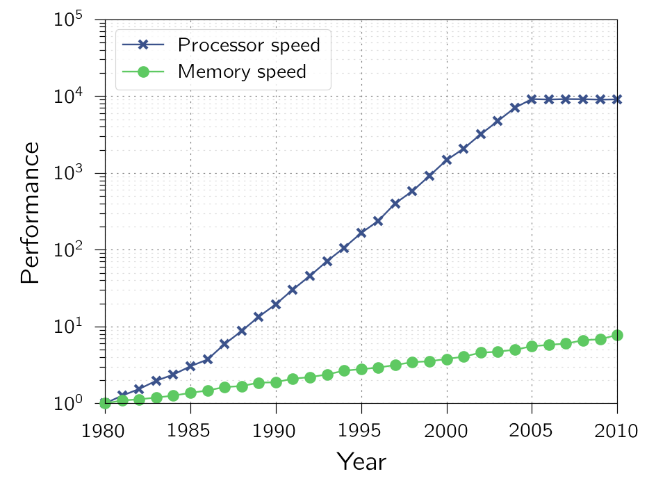{width=70%}
:::{.smaller}
Based on figure from "Computer Architecture" by _J. Hennessy_ and _D. Patterson_
:::
## Access time example (1/2) {.leftalign}
<!--
File `data.py`:
```{.python}
import time
import pickle
import numpy as np
def create_random_data():
np.random.seed(3922)
start = time.perf_counter()
data = np.random.randint(0, 2**20, size=(128, 128, 128, 128))
end = time.perf_counter()
print('{:10.5f}: Create "random" data'.format(end-start))
return data
def create_42_data():
start = time.perf_counter()
data = np.full((128, 128, 128, 128), 42)
end = time.perf_counter()
print('{:10.5f}: Create "42" data'.format(end-start))
return data
def store_data(filename, data, dataname):
start = time.perf_counter()
with open(filename, 'wb') as outfile:
pickle.dump(data, outfile)
end = time.perf_counter()
print('{:10.5f}: Store "{:s}" data'.format(end-start, dataname))
def load_data(filename, dataname):
start = time.perf_counter()
with open(filename, 'rb') as infile:
data = pickle.load(infile)
end = time.perf_counter()
print('{:10.5f}: Load "{:s}" data'.format(end-start, dataname))
return data
def operate_on_data(data, dataname):
start = time.perf_counter()
new_data = data + 1.1
end = time.perf_counter()
print('{:10.5f}: Operate on "{:s}" data'.format(end-start, dataname))
return new_data
```
File `save_it.py`:
```{.python}
from data import *
dataname = 'random'
data = create_random_data()
store_data(filename='temp01.dat',
data=data, dataname=dataname)
dataname = '42'
data = create_42_data()
store_data(filename='temp02.dat',
data=data, dataname=dataname)
```
File `from_disk.py`:
```{.python}
from data import *
dataname = 'random'
data = load_data(filename='temp01.dat',
dataname=dataname)
new_data = operate_on_data(data=data,
dataname=dataname)
dataname = '42'
data = load_data(filename='temp02.dat',
dataname=dataname)
new_data = operate_on_data(data=data,
dataname=dataname)
```
File `in_memory.py`:
```{.python}
from data import *
dataname = 'random'
data = create_random_data()
new_data = operate_on_data(data=data,
dataname=dataname)
dataname = '42'
data = create_42_data()
new_data = operate_on_data(data=data,
dataname=dataname)
```
-->
| | Levante (Fixed) | Local (Fixed) | Levante (Random) | Local (Random) |
| -------------------------- | ----------------- | ----------------- | ----------------- | ----------------- |
| Create data | 0.5607 | 0.2280 | 1.6623 | 0.8759 |
| Load data | 0.7605 | 0.8767 | 0.7615 | 0.9225 |
| Store data | 2.2317 | 4.0427 | 2.2327 | 3.4378 |
| Process data | 0.7618 | 0.3792 | 0.7572 | 0.3747 |
:::{.smaller}
Time in seconds using a 2 GB numpy array ($128 \times 128 \times 128 \times 128$) either with a fixed number or random number in each entry
:::
## Access time example (2/2) {.leftalign}
- Reading/writing to file is rather expensive
- If necessary during computation, try doing it asynchronously
- If possible, keep data in memory
## Techniques
- Caching
- Prefetching
- Branch prediction
## Unavailable data
If data is not available in the current memory level
- register spilling (register -> cache)
- cache missing (cache -> main memory)
- page fault (main memory -> disk)
Miss description
## External Memory Model
balance block size to get from next level to latency it takes to get it
## Memory access time model (1/3)
| Cache | Access Time | Hit Ratio |
| ------ | ------------ | ---------- |
| $L_1$ | $T_1$ | $H_1$ |
| $L_2$ | $T_2$ | |
- Parallel and serial requests possible
## Memory access time model (2/3)
| Cache | Access Time | Hit Ratio |
| ------ | ------------ | ---------- |
| $L_1$ | $T_1$ | $H_1$ |
| $L_2$ | $T_2$ | $H_2$ |
| $L_3$ | $T_3$ | |
## Memory access time model (3/3)
- Average memory access time $T_{avg,p}$ for parallel access (processor connected to all caches)
:::{.smaller}
\begin{align}
T_{avg,p} &= H_1 T_1 + ((1-H_1)\cdot H_2)\cdot T_2\\
&+ ((1-H_1)\cdot(1-H_2))\cdot T_3
\end{align}
:::
- Average memory access time $T_{avg,s}$ for serial access
:::{.smaller}
\begin{align}
T_{avg,s} &= H_1 T_1 + ((1-H_1)\cdot H_2)\cdot(T_1+T_2)\\
&+ ((1-H_1)\cdot(1-H_2))\cdot(T_1+T_2+T_3)
\end{align}
:::
## Overview/Exercise
- Introduction from base of pyramid (file access)
- example with access from disk and directly from memory
- background on memory hierarchy with focus on today instead of history
- Working our way up the pyramid
- reference values for Levante CPU
- example with optimal and sub-optimal memory access, i.e. cache blocking (see `nproma`)
- openmp reduction (hand implementation), reference/continuation from parallelism lecture
## Observations
- Gap between processor and memory speeds.
Hierarchy needed because of discrepancy between speed of CPU and (main) memory
(include image)
- exploit accessing data and code stored close to each other (temporal and spatial locality)
## Memory Pyramid (upwards)
:::{.r-stack}
{.fragment width=70% fragment-index=1}
{.fragment width=70% fragment-index=2}
{.fragment width=70% fragment-index=3}
{.fragment width=70% fragment-index=4}
{.fragment width=70% fragment-index=5}
{.fragment width=70% fragment-index=6}
:::
## Memory Pyramid (downwards) - check numbers {auto-animate=true}
Order of magnitude on Levante (AMD EPYC 7763)
- Base frequency: 2.45 GHz
## Memory Pyramid (downwards) - check numbers {auto-animate=true}
Order of magnitude on Levante (AMD EPYC 7763)
Access time (ns) Capacity
------------ ----------------- ---------
Register ~0.4 1 KB
:::{.incremental}
- L1 Cache about 3 times slower
:::
## Memory Pyramid (downwards) - check numbers {auto-animate=true}
Order of magnitude on Levante (AMD EPYC 7763)
Access time (ns) Capacity
------------ ----------------- ---------
Register ~0.4 1 KB
L1 Cache ~1.1 32 KB
:::{.incremental}
- Same factors for L2 and L3
:::
## Memory Pyramid (downwards) - check numbers {auto-animate=true}
Order of magnitude on Levante (AMD EPYC 7763)
Access time (ns) Capacity
------------ ----------------- ---------
Register ~0.4 1 KB
L1 Cache ~1.1 32 KB
L2 Cache ~3.3 512 KB
L3 Cache ~12.8 32 MB
:::{.incremental}
- 256 GB of main memory (default) with a theoretical memory bandwidth of ~200 GB/s
:::
## Memory Pyramid (downwards) - check numbers {auto-animate=true}
Order of magnitude on Levante (AMD EPYC 7763)
Access time (ns) Capacity
------------ ----------------- ---------
Register ~0.4 1 KB
L1 Cache ~1.1 32 KB
L2 Cache ~3.3 512 KB
L3 Cache ~12.8 32 MB
Main Memory 60 256 GB
:::{.incremental}
- Fast Data as Flash based file system
:::
## Memory Pyramid (downwards) - check numbers {auto-animate=true}
Order of magnitude on Levante (AMD EPYC 7763)
Access time (ns) Capacity
------------ ----------------- ---------
Register ~0.4 1 KB
L1 Cache ~1.1 32 KB
L2 Cache ~3.3 512 KB
L3 Cache ~12.8 32 MB
Main Memory 60 256 GB
SSD 100 1 PB
:::{.incremental}
- File system at Levante ~130 PB, limited by quota for project
:::
## Memory Pyramid (downwards) - check numbers {auto-animate=true}
Order of magnitude on Levante (AMD EPYC 7763)
Access time (ns) Capacity
------------ ----------------- ---------
Register ~0.4 1 KB
L1 Cache ~1.1 32 KB
L2 Cache ~3.3 512 KB
L3 Cache ~12.8 32 MB
Main Memory ~60 256 GB
SSD ~100 1 PB
Hard disk ~3000 130 PB
:::{.incremental}
- Tape backup also possible
:::
## Memory Mountain (1/2)
Describe what is done
- Influence of block size
- Influence of stride
- Measurements done on Levante compute node
## Memory Mountain (2/2)
:::{r-stack}
{width=70%}
:::
:::{.smaller}
$\approx$ Factor 20 between best and worst access
:::
## Different architectures
- Different caches are available
- Speed and size of caches varies
- Basic understanding helps in all cases
- Hardware-specific knowledge allows additional fine-tuning
# Resources {.leftalign}
- "Computer Systems: A Programmer's Perspective" by _R. Bryant_ and _D. O'Hallaron_, Pearson
- "Computer Architecture" by _J. Hennessy_ and _D. Patterson_, O'Reilly